Two basic concepts, future value and present value, were introduced in the beginning of this chapter. With a 10 percent interest rate, an investor with $1 today can generate a future value of $1.10 in a year, $1.21 [= $1 x (1.10)2] in two years, and so on. Conversely, present value analysis places a current value on a future cash flow. With the same 10 percent interest rate, a dollar to be received in one year has a present value of $0.909 (= $1/1.10) in year 0. A dollar to be received in two years has a present value of $0.826 [= $1/(1.10)2].
We commonly express an interest rate as, say, 12 percent per year. However, we can speak of the interest rate as 3 percent per quarter. Although the stated annual interest rate remains 12 percent (= 3 percent x 4), the effective annual interest rate is 12.55 percent [= (1.03)4 - 1]. In other words, the compounding process increases the future value of an investment. The limiting case is continuous compounding, where funds are assumed to be reinvested every infinitesimal instant.
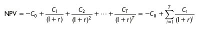
A basic quantitative technique for financial decision making is net present value analysis. The net present value formula for an investment that generates cash flows (Ci) in future periods is:
The formula assumes that the cash flow at date 0 is the initial investment (a cash outflow).
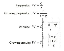
Frequently, the actual calculation of present value is long and tedious. The computation of the present value of a long-term mortgage with monthly payments is a good example of this. We presented four simplifying formulas:
We stressed a few practical considerations in the application of these formulas:
The numerator in each of the formulas, C, is the cash flow to be received one full period hence.
Cash flows are generally irregular in practice. To avoid unwieldy problems, assumptions to create more regular cash flows are made both in this textbook and in the real world.
A number of present value problems involve annuities (or perpetuities) beginning a few periods hence. Students should practice combining the annuity (or perpetuity) formula with the discounting formula to solve these problems.
Annuities and perpetuities may have periods of every two or every n years, rather than once a year. The annuity and perpetuity formulas can easily handle such circumstances.
We frequently encounter problems where the present value of one annuity must be equated with the present value of another annuity.