In Chaps. 16 and 17 we were concerned with the plane motion of
rigid bodies and of systems of rigid bodies. In Chap. 16 and in the
second half of Chap. 17 (momentum method), our study was further
restricted to that of plane slabs and of bodies symmetrical with respect
to the reference plane. However, many of the fundamental results
obtained in these two chapters remain valid in the case of the motion
of a rigid body in three dimensions.
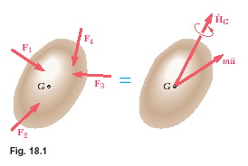
For example, the two fundamental equations
 <a onClick="window.open('/olcweb/cgi/pluginpop.cgi?it=jpg:: ::/sites/dl/free/007230491x/60491/chap18equA.jpg','popWin', 'width=313,height=120,resizable,scrollbars');" href="#"><img valign="absmiddle" height="16" width="16" border="0" src="/olcweb/styles/shared/linkicons/image.gif"> (4.0K)</a> <a onClick="window.open('/olcweb/cgi/pluginpop.cgi?it=jpg:: ::/sites/dl/free/007230491x/60491/chap18equA.jpg','popWin', 'width=313,height=120,resizable,scrollbars');" href="#"><img valign="absmiddle" height="16" width="16" border="0" src="/olcweb/styles/shared/linkicons/image.gif"> (4.0K)</a>
on which the analysis of the plane motion of a rigid body was based,
remain valid in the most general case of motion of a rigid body. As
indicated in Sec. 16.2, these equations express that the system of the
external forces is equipollent to the system consisting of the vector
 <a onClick="window.open('/olcweb/cgi/pluginpop.cgi?it=jpg:: ::/sites/dl/free/007230491x/60491/chap18equB.jpg','popWin', 'width=77,height=92,resizable,scrollbars');" href="#"><img valign="absmiddle" height="16" width="16" border="0" src="/olcweb/styles/shared/linkicons/image.gif"> (0.0K)</a>
attached at G and the couple of moment <a onClick="window.open('/olcweb/cgi/pluginpop.cgi?it=jpg:: ::/sites/dl/free/007230491x/60491/chap18equB.jpg','popWin', 'width=77,height=92,resizable,scrollbars');" href="#"><img valign="absmiddle" height="16" width="16" border="0" src="/olcweb/styles/shared/linkicons/image.gif"> (0.0K)</a>
attached at G and the couple of moment
 <a onClick="window.open('/olcweb/cgi/pluginpop.cgi?it=jpg:: ::/sites/dl/free/007230491x/60491/chap18equC.jpg','popWin', 'width=78,height=93,resizable,scrollbars');" href="#"><img valign="absmiddle" height="16" width="16" border="0" src="/olcweb/styles/shared/linkicons/image.gif"> (0.0K)</a>
(Fig. 18.1). <a onClick="window.open('/olcweb/cgi/pluginpop.cgi?it=jpg:: ::/sites/dl/free/007230491x/60491/chap18equC.jpg','popWin', 'width=78,height=93,resizable,scrollbars');" href="#"><img valign="absmiddle" height="16" width="16" border="0" src="/olcweb/styles/shared/linkicons/image.gif"> (0.0K)</a>
(Fig. 18.1). However, the relation
 <a onClick="window.open('/olcweb/cgi/pluginpop.cgi?it=jpg:: ::/sites/dl/free/007230491x/60491/chap18equD.jpg','popWin', 'width=116,height=93,resizable,scrollbars');" href="#"><img valign="absmiddle" height="16" width="16" border="0" src="/olcweb/styles/shared/linkicons/image.gif"> (1.0K)</a>
which enabled us to determine the angular momentum of a rigid slab and which played an important part in the solution of problems involving the plane motion of slabs and bodies symmetrical with respect to the reference plane, ceases to be valid in the case of nonsymmetrical bodies or three-dimensional
motion. Thus in the first part of the chapter, in Sec. 18.2, a more general
method for computing the angular momentum HG of a rigid body
in three dimensions will be developed. <a onClick="window.open('/olcweb/cgi/pluginpop.cgi?it=jpg:: ::/sites/dl/free/007230491x/60491/chap18equD.jpg','popWin', 'width=116,height=93,resizable,scrollbars');" href="#"><img valign="absmiddle" height="16" width="16" border="0" src="/olcweb/styles/shared/linkicons/image.gif"> (1.0K)</a>
which enabled us to determine the angular momentum of a rigid slab and which played an important part in the solution of problems involving the plane motion of slabs and bodies symmetrical with respect to the reference plane, ceases to be valid in the case of nonsymmetrical bodies or three-dimensional
motion. Thus in the first part of the chapter, in Sec. 18.2, a more general
method for computing the angular momentum HG of a rigid body
in three dimensions will be developed.
|  <a onClick="window.open('/olcweb/cgi/pluginpop.cgi?it=jpg:: ::/sites/dl/free/007230491x/60491/chap18figA.jpg','popWin', 'width=324,height=254,resizable,scrollbars');" href="#"><img valign="absmiddle" height="16" width="16" border="0" src="/olcweb/styles/shared/linkicons/image.gif"> (11.0K)</a> <a onClick="window.open('/olcweb/cgi/pluginpop.cgi?it=jpg:: ::/sites/dl/free/007230491x/60491/chap18figA.jpg','popWin', 'width=324,height=254,resizable,scrollbars');" href="#"><img valign="absmiddle" height="16" width="16" border="0" src="/olcweb/styles/shared/linkicons/image.gif"> (11.0K)</a> |
Similarly, although the main feature of the impulse-momentum
method discussed in Sec. 17.7, namely, the reduction of the momenta
of the particles of a rigid body to a linear momentum vector
 <a onClick="window.open('/olcweb/cgi/pluginpop.cgi?it=jpg:: ::/sites/dl/free/007230491x/60491/chap18equE.jpg','popWin', 'width=78,height=88,resizable,scrollbars');" href="#"><img valign="absmiddle" height="16" width="16" border="0" src="/olcweb/styles/shared/linkicons/image.gif"> (0.0K)</a>
attached at the mass center G of the body and an angular momentum
couple HG, remains valid, the relation <a onClick="window.open('/olcweb/cgi/pluginpop.cgi?it=jpg:: ::/sites/dl/free/007230491x/60491/chap18equE.jpg','popWin', 'width=78,height=88,resizable,scrollbars');" href="#"><img valign="absmiddle" height="16" width="16" border="0" src="/olcweb/styles/shared/linkicons/image.gif"> (0.0K)</a>
attached at the mass center G of the body and an angular momentum
couple HG, remains valid, the relation
<a onClick="window.open('/olcweb/cgi/pluginpop.cgi?it=jpg:: ::/sites/dl/free/007230491x/60491/chap18equD.jpg','popWin', 'width=116,height=93,resizable,scrollbars');" href="#"><img valign="absmiddle" height="16" width="16" border="0" src="/olcweb/styles/shared/linkicons/image.gif"> (1.0K)</a>
must be discarded and replaced by the more general relation developed in Sec. 18.2 before this method can be applied to the three-dimensional motion of
a rigid body (Sec. 18.3).
We also note that the work-energy principle (Sec. 17.2) and the
principle of conservation of energy (Sec. 17.6) still apply in the case
of the motion of a rigid body in three dimensions. However, the expression obtained in Sec. 17.4 for the kinetic energy of a rigid body
in plane motion will be replaced by a new expression developed in
Sec. 18.4 for a rigid body in three-dimensional motion.
In the second part of the chapter, you will first learn to determine
the rate of change
<a onClick="window.open('/olcweb/cgi/pluginpop.cgi?it=jpg:: ::/sites/dl/free/007230491x/60491/chap18equC.jpg','popWin', 'width=78,height=93,resizable,scrollbars');" href="#"><img valign="absmiddle" height="16" width="16" border="0" src="/olcweb/styles/shared/linkicons/image.gif"> (0.0K)</a>
of the angular momentum HG of a threedimensional
rigid body, using a rotating frame of reference with respect
to which the moments and products of inertia of the body remain
constant (Sec. 18.5). Equations (18.1) and (18.2) will then be expressed
in the form of free-body-diagram equations, which can be
used to solve various problems involving the three-dimensional motion
of rigid bodies (Secs. 18.6 through 18.8).
The last part of the chapter (Secs. 18.9 through 18.11) is devoted
to the study of the motion of the gyroscope or, more generally, of an
axisymmetrical body with a fixed point located on its axis of symmetry.
In Sec. 18.10, the particular case of the steady precession of a
gyroscope will be considered, and, in Sec. 18.11, the motion of an
axisymmetrical body subjected to no force, except its own weight, will
be analyzed.
|