 |  Statistics for the Behavioral Sciences, 4/e Michael Thorne,
Mississippi State University -- Mississippi State
Martin Giesen,
Mississippi State University -- Mississippi State
One-Way Analysis of Variance With Post Hoc Comparisons
SPSS ExercisesUSING SPSS-EXAMPLES AND EXERCISES
SPSS has several techniques for performing analysis of variance (ANOVA). The ONEWAY procedure is
one such method, and it will perform a variety of post hoc tests. For the repeated measures ANOVA, we
will need to use the SPSS GLM (General Linear Model)-Repeated Measures procedure to obtain the
analysis. The SPSS GLM procedures will perform analyses for many different types of ANOVA designs.
Unfortunately-given our desire to keep this as simple as possible-the SPSS GLM procedures are some
of the "fancier" SPSS techniques and provide extensive output that is well beyond the level of the textbook.Example-Independent Groups ANOVA: As an example of an independent groups ANOVA, we will
work Problem 1 using SPSS. We will illustrate how to perform the ANOVA, how to do the LSD and HSD
post hoc tests, how to graph the means, and how to provide an Error Bar chart of the groups. The steps are
as follows:- Start SPSS and enter the data. The data entry is an extension of the set-up we used for the two-sample independent-groups t test. Name the two variables group and distance. The group variable will have a 1 entered for each distance score from Group 1, a 2 for each distance score from Group 2, and so on.
- Select Analyze > Compare Means > One-Way ANOVA.
- Move distance to the Dependent List box because it is the dependent variable. Move group to the Factor box.
- Select the Post Hoc box and choose LSD and Tukey (HSD) in the Post Hoc Multiple Comparisons box. Then select Continue.
- Select the Options box; click Descriptive and Means plot (this will give you a line graph of the group means), then Continue > OK. The results should appear in the output Viewer window.
- As an extra illustration for this exercise, we will create an Error Bar chart for the groups, which shows a plot of the confidence intervals for each group. This type of graph is helpful in understanding and emphasizing that there is within-group variability that is not shown in graphs of group means as point estimates.
- Select Graphs>Error Bar > Simple > Summaries for groups of cases > Define
.
- Move distance into the Variable box and move group into the Category Axis box. Other settings in this dialog box should indicate a 95% confidence interval for means. Next click OK, and the graph should appear in the output Viewer window.
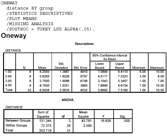
Notes on Reading the Output- The ANOVA output box gives the source table. The "Sig." after the F value is the exact probability value for the obtained F ratio. For example, p = .000 means that p is 0 when rounded to three decimal places. Because p is never exactly 0, it is better to express this probability as p < .001.
- The Multiple Comparisons box is highly redundant. It does not give a test statistic value for each comparison or a minimum difference required for significance between two groups. Instead the box indicates the significant comparisons by an asterisk beside the Mean Difference and the exact p value given in the Sig. column. For example, the Tukey HSD results indicate that Group 1 versus Group 4 and Group 2 versus Group 3 are the only comparisons that are not statistically different. The more powerful LSD test indicates that only Groups 1 and 4 are not statistically different.
- The Means Plots and the Graph showing confidence intervals provide pictures of the results. Because their confidence intervals overlap considerably, we would expect Groups 1 and 4 and Groups 2 and 3 not to be statistically different. Of course, this is what we found with the HSD test.
 <a onClick="window.open('/olcweb/cgi/pluginpop.cgi?it=gif:: ::/sites/dl/free/0072832517/55320/c11_spss1.gif','popWin', 'width=NaN,height=NaN,resizable,scrollbars');" href="#"><img valign="absmiddle" height="16" width="16" border="0" src="/olcweb/styles/shared/linkicons/image.gif"> (18.0K)</a> <a onClick="window.open('/olcweb/cgi/pluginpop.cgi?it=gif:: ::/sites/dl/free/0072832517/55320/c11_spss1.gif','popWin', 'width=NaN,height=NaN,resizable,scrollbars');" href="#"><img valign="absmiddle" height="16" width="16" border="0" src="/olcweb/styles/shared/linkicons/image.gif"> (18.0K)</a> 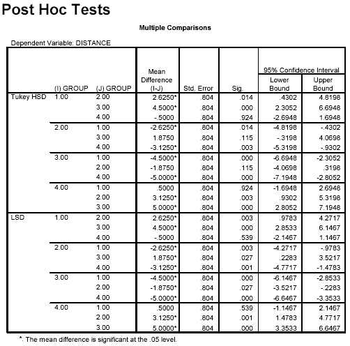 <a onClick="window.open('/olcweb/cgi/pluginpop.cgi?it=gif:: ::/sites/dl/free/0072832517/55320/c11_spss2.gif','popWin', 'width=NaN,height=NaN,resizable,scrollbars');" href="#"><img valign="absmiddle" height="16" width="16" border="0" src="/olcweb/styles/shared/linkicons/image.gif"> (23.0K)</a> <a onClick="window.open('/olcweb/cgi/pluginpop.cgi?it=gif:: ::/sites/dl/free/0072832517/55320/c11_spss2.gif','popWin', 'width=NaN,height=NaN,resizable,scrollbars');" href="#"><img valign="absmiddle" height="16" width="16" border="0" src="/olcweb/styles/shared/linkicons/image.gif"> (23.0K)</a> 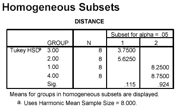 <a onClick="window.open('/olcweb/cgi/pluginpop.cgi?it=gif:: ::/sites/dl/free/0072832517/55320/c11_spss3.gif','popWin', 'width=NaN,height=NaN,resizable,scrollbars');" href="#"><img valign="absmiddle" height="16" width="16" border="0" src="/olcweb/styles/shared/linkicons/image.gif"> (9.0K)</a> <a onClick="window.open('/olcweb/cgi/pluginpop.cgi?it=gif:: ::/sites/dl/free/0072832517/55320/c11_spss3.gif','popWin', 'width=NaN,height=NaN,resizable,scrollbars');" href="#"><img valign="absmiddle" height="16" width="16" border="0" src="/olcweb/styles/shared/linkicons/image.gif"> (9.0K)</a> 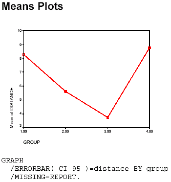 <a onClick="window.open('/olcweb/cgi/pluginpop.cgi?it=gif:: ::/sites/dl/free/0072832517/55320/c11_spss4.gif','popWin', 'width=NaN,height=NaN,resizable,scrollbars');" href="#"><img valign="absmiddle" height="16" width="16" border="0" src="/olcweb/styles/shared/linkicons/image.gif"> (6.0K)</a> <a onClick="window.open('/olcweb/cgi/pluginpop.cgi?it=gif:: ::/sites/dl/free/0072832517/55320/c11_spss4.gif','popWin', 'width=NaN,height=NaN,resizable,scrollbars');" href="#"><img valign="absmiddle" height="16" width="16" border="0" src="/olcweb/styles/shared/linkicons/image.gif"> (6.0K)</a> 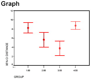 <a onClick="window.open('/olcweb/cgi/pluginpop.cgi?it=gif:: ::/sites/dl/free/0072832517/55320/c11_spss5.gif','popWin', 'width=NaN,height=NaN,resizable,scrollbars');" href="#"><img valign="absmiddle" height="16" width="16" border="0" src="/olcweb/styles/shared/linkicons/image.gif"> (3.0K)</a> Example-Repeated Measures ANOVA: Our example of the repeated measures ANOVA will use the
SPSS GLM-Repeated Measures procedure. This technique will perform the analysis for the one-way
repeated measures exercises in the text and in this study guide in addition to analyzing more extensive
designs. The procedure does not do post hoc tests for this completely within-subjects design, so we will not
be concerned with this part of our computer solution. The supplemental text on using SPSS suggested in
Appendix 4 explains how to do such tests. (In short, the post hoc tests are performed by computing
sequential pairwise dependent t tests and testing for significance by using the α level obtained by dividing
.05 by the number of tests performed.) Alternatively, you can compute the post hoc tests by hand, using
information from the output and the procedures described in the text. We will solve Problem 6 as an
example. Here are the steps to follow: <a onClick="window.open('/olcweb/cgi/pluginpop.cgi?it=gif:: ::/sites/dl/free/0072832517/55320/c11_spss5.gif','popWin', 'width=NaN,height=NaN,resizable,scrollbars');" href="#"><img valign="absmiddle" height="16" width="16" border="0" src="/olcweb/styles/shared/linkicons/image.gif"> (3.0K)</a> Example-Repeated Measures ANOVA: Our example of the repeated measures ANOVA will use the
SPSS GLM-Repeated Measures procedure. This technique will perform the analysis for the one-way
repeated measures exercises in the text and in this study guide in addition to analyzing more extensive
designs. The procedure does not do post hoc tests for this completely within-subjects design, so we will not
be concerned with this part of our computer solution. The supplemental text on using SPSS suggested in
Appendix 4 explains how to do such tests. (In short, the post hoc tests are performed by computing
sequential pairwise dependent t tests and testing for significance by using the α level obtained by dividing
.05 by the number of tests performed.) Alternatively, you can compute the post hoc tests by hand, using
information from the output and the procedures described in the text. We will solve Problem 6 as an
example. Here are the steps to follow:- Start SPSS and name the variables day1, wk3, wk6, and wk9. Enter the data for each of these variables. Note that this data entry arrangement is an extension of the arrangement used for the pairedsamples t test. Each participant's data are given on one row.
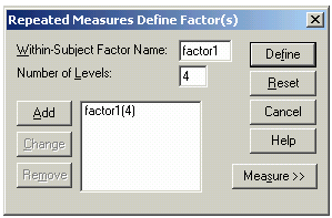
- Select Analyze > General Linear Model > GLM-Repeated Measures.
- In the dialog box, enter the number of levels (4 for the four times of measurement), and click Add. The Define Factor(s) dialog box should appear as follows. Then select Define.
 <a onClick="window.open('/olcweb/cgi/pluginpop.cgi?it=gif:: ::/sites/dl/free/0072832517/55320/c11_spss6.gif','popWin', 'width=NaN,height=NaN,resizable,scrollbars');" href="#"><img valign="absmiddle" height="16" width="16" border="0" src="/olcweb/styles/shared/linkicons/image.gif"> (8.0K)</a> <a onClick="window.open('/olcweb/cgi/pluginpop.cgi?it=gif:: ::/sites/dl/free/0072832517/55320/c11_spss6.gif','popWin', 'width=NaN,height=NaN,resizable,scrollbars');" href="#"><img valign="absmiddle" height="16" width="16" border="0" src="/olcweb/styles/shared/linkicons/image.gif"> (8.0K)</a> - In the GLM-Repeated Measures dialog box, highlight each of the variables and move them into the Within-Subjects Variables box in order-that is, day1 is first and wk9 is fourth. The dialog box should appear as follows:
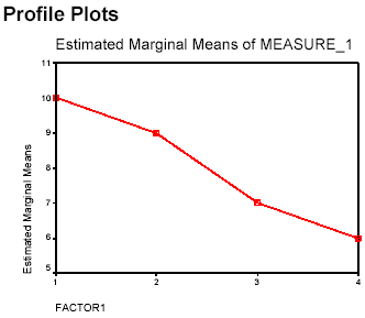
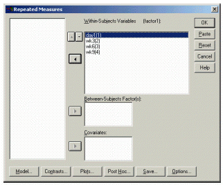 <a onClick="window.open('/olcweb/cgi/pluginpop.cgi?it=gif:: ::/sites/dl/free/0072832517/55320/c11_spss7.gif','popWin', 'width=NaN,height=NaN,resizable,scrollbars');" href="#"><img valign="absmiddle" height="16" width="16" border="0" src="/olcweb/styles/shared/linkicons/image.gif"> (28.0K)</a> <a onClick="window.open('/olcweb/cgi/pluginpop.cgi?it=gif:: ::/sites/dl/free/0072832517/55320/c11_spss7.gif','popWin', 'width=NaN,height=NaN,resizable,scrollbars');" href="#"><img valign="absmiddle" height="16" width="16" border="0" src="/olcweb/styles/shared/linkicons/image.gif"> (28.0K)</a> - Although it is not required for the analysis, we will also get a plot of the means by selecting the Plots box, highlighting "factor 1" and moving it to the Horizontal Axis box, then clicking Add > Continue.
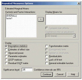
- We want descriptive statistics for our groups, so select Options, then click on Descriptive Statistics in the Options dialog box, which should appear as follows. Click on Continue.
 <a onClick="window.open('/olcweb/cgi/pluginpop.cgi?it=gif:: ::/sites/dl/free/0072832517/55320/c11_spss8.gif','popWin', 'width=NaN,height=NaN,resizable,scrollbars');" href="#"><img valign="absmiddle" height="16" width="16" border="0" src="/olcweb/styles/shared/linkicons/image.gif"> (32.0K)</a> <a onClick="window.open('/olcweb/cgi/pluginpop.cgi?it=gif:: ::/sites/dl/free/0072832517/55320/c11_spss8.gif','popWin', 'width=NaN,height=NaN,resizable,scrollbars');" href="#"><img valign="absmiddle" height="16" width="16" border="0" src="/olcweb/styles/shared/linkicons/image.gif"> (32.0K)</a> - You should now be back to the GLM-Repeated Measures dialog box. Click OK, and the results should appear in the output Viewer window.
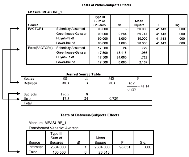
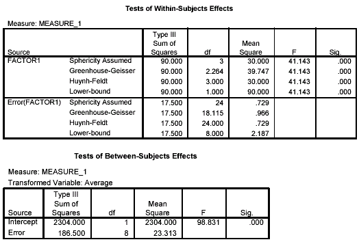
Notes on Reading the Output- As you learn to use statistical software, one skill that you will need to develop is the ability to ignore parts of the output that are superfluous for what you are trying to do. You will also need to learn to focus on the important and necessary parts of the output for your particular problem. In fact, both of these skills are necessary for you to extract the information from the output that you need for solving the present exercise.
- In the following output, we have included only the portions that are needed for the present exercise. Your task is to ignore other parts of the output that are produced by the process we have described.
- The Descriptive Statistics box gives exactly that information.
- Locate the box labeled Tests of Within-Subjects Effects. Also locate the box labeled Tests of Between-Subjects Effects. The following figure shows the information needed from these two boxes to construct the source table needed for this exercise.
 <a onClick="window.open('/olcweb/cgi/pluginpop.cgi?it=gif:: ::/sites/dl/free/0072832517/55320/c11_spss9.gif','popWin', 'width=NaN,height=NaN,resizable,scrollbars');" href="#"><img valign="absmiddle" height="16" width="16" border="0" src="/olcweb/styles/shared/linkicons/image.gif"> (22.0K)</a> <a onClick="window.open('/olcweb/cgi/pluginpop.cgi?it=gif:: ::/sites/dl/free/0072832517/55320/c11_spss9.gif','popWin', 'width=NaN,height=NaN,resizable,scrollbars');" href="#"><img valign="absmiddle" height="16" width="16" border="0" src="/olcweb/styles/shared/linkicons/image.gif"> (22.0K)</a>  <a onClick="window.open('/olcweb/cgi/pluginpop.cgi?it=gif:: ::/sites/dl/free/0072832517/55320/c11_spss10.gif','popWin', 'width=NaN,height=NaN,resizable,scrollbars');" href="#"><img valign="absmiddle" height="16" width="16" border="0" src="/olcweb/styles/shared/linkicons/image.gif"> (13.0K)</a> <a onClick="window.open('/olcweb/cgi/pluginpop.cgi?it=gif:: ::/sites/dl/free/0072832517/55320/c11_spss10.gif','popWin', 'width=NaN,height=NaN,resizable,scrollbars');" href="#"><img valign="absmiddle" height="16" width="16" border="0" src="/olcweb/styles/shared/linkicons/image.gif"> (13.0K)</a>
 <a onClick="window.open('/olcweb/cgi/pluginpop.cgi?it=gif:: ::/sites/dl/free/0072832517/55320/c11_spss11.gif','popWin', 'width=NaN,height=NaN,resizable,scrollbars');" href="#"><img valign="absmiddle" height="16" width="16" border="0" src="/olcweb/styles/shared/linkicons/image.gif"> (16.0K)</a> <a onClick="window.open('/olcweb/cgi/pluginpop.cgi?it=gif:: ::/sites/dl/free/0072832517/55320/c11_spss11.gif','popWin', 'width=NaN,height=NaN,resizable,scrollbars');" href="#"><img valign="absmiddle" height="16" width="16" border="0" src="/olcweb/styles/shared/linkicons/image.gif"> (16.0K)</a>
 <a onClick="window.open('/olcweb/cgi/pluginpop.cgi?it=gif:: ::/sites/dl/free/0072832517/55320/c11_spss12.gif','popWin', 'width=NaN,height=NaN,resizable,scrollbars');" href="#"><img valign="absmiddle" height="16" width="16" border="0" src="/olcweb/styles/shared/linkicons/image.gif"> (5.0K)</a> <a onClick="window.open('/olcweb/cgi/pluginpop.cgi?it=gif:: ::/sites/dl/free/0072832517/55320/c11_spss12.gif','popWin', 'width=NaN,height=NaN,resizable,scrollbars');" href="#"><img valign="absmiddle" height="16" width="16" border="0" src="/olcweb/styles/shared/linkicons/image.gif"> (5.0K)</a> Exercises Using SPSS - Work Self-Test Exercise 4 using SPSS. Obtain LSD post hoc test results and an Error Bar graph of the 95% confidence intervals for each group. Write a complete conclusion for the ANOVA and LSD test.
- Work Problem 8 using SPSS with the GLM-Repeated Measures procedure. Obtain a plot of the means and use the output to construct the desired source table.
 Click here to view the answers. (161.0K) Click here to view the answers. (161.0K)
|
|


 2003 McGraw-Hill Higher Education