Project Examples

Presenting the Results

Payday Nuts Observational Study

Payday candy bars consist of caramel and nuts. Many people enjoy having a regular size, 52_g, or a king size, 96_g, Payday candy bar as a snack. Our group wanted to see what percent of Payday candy bars are nuts. In addition, we wanted to know how the size of the candy bar would affect the amount of nuts.

The population that we sampled was all Payday candy bars weighing both 52_g and 96_g. The sampling was done by randomly selecting the stores in towns of our choice. The towns of our choice were Lincoln, Auburn, Nebraska City and Peru. We chose these towns because someone out of our group would be in that town before we conducted our data collection process. We listed some of the convenience stores from each of these towns. We labeled each store from 01 to 20 then went to table A and selected eight stores. The following list of stores were our sample set: Super C, Amoco, and Gas and Shop in Lincoln, Casey’s and Texaco in Auburn, Quick Pick and Taylor’s Quick Shop in Nebraska City, and Casey’s and Decker’s in Peru. As each participant went to the different locations, they flipped a coin to randomly select which candy bars from each store we would purchase. If the coin showed heads, he/she would take a candy bar from the top. If the coin showed tails, he/she would take a candy bar from the bottom of the stack. This was done for both regular size and king size candy bars.

To measure the items, we used a scale from the Science department. To ensure that the scale was accurate we measured a weight that we already knew was accurate. Then to ensure that the weights of the nuts and caramel were accurate we had more than one person weigh each one. We measured the weight of nuts accurate to the nearest hundredth. In the actual process of removing the nuts from the caramel we all worked on it as accurately as possible. In some cases it was hard to separate the nuts from the caramel and vice versa.

We have a few variables in our study. One variable in our study was size. We will compare percentages with a regular size Payday, 52_g, and a king size Payday, 96_g. Another variable is the weight of nuts in each candy bar. The weight of the nuts was our explanatory variable. The random selection of stores we purchased the candy bars from and the different towns varied but are not the actual variables; they are the randomness of our project. The randomness comes into play in the sampling process. We randomly selected the stores in towns of our choice.

To ensure accuracy we had the weight of the nuts measured by more than one person in our group. Accuracy has two aspects, lack of bias and reliability. A measurement is to have both small bias and high reliability. Each individual weighed the nuts several times to improve reliability. The scales in the science lab had small bias because when we weighed a 2 pound weight it was not erratic in its results. The result was consistent at 2 pounds. Since we know no measuring process is perfectly reliable, we used the average of the several repeated measurements of the nuts for each candy bar. As long as we insured accuracy the data was relatively easy to collect, therefore, it was simple data. These charts show the results of our data collection.

The information gathered from these charts shows us that the regular size Payday candy bar has a mean of .4733, which is 47.33 percent nuts, and a standard deviation of .0185. The result of standard deviation shows that the data is very close together. The king size Payday candy bar was relatively close, with a mean of .4694, which is 46.94 percent nuts, and a standard deviation of .0212.

This box plot shows this information graphically. As one can see the standard deviation shows that the data was all close together.

The test of significance is designed to assess the strength of the data against the null hypothesis. A test of significance assesses this in terms of probability. In this study our null hypothesis or H₀ states that the percentage of nuts for all 52_g candy bars is equal to the percentage for all 96_g candy bars.

The other statement being tested in a test of significance is called the alternative hypothesis or H_a. In our study this statement states that the percentage of nuts in 52_g candy bars does not equal the percentage of nuts in 96_g candy bars. The H₀ is proven to be true as our P-Value of .74. The P-Value is the probability that the test statistic would take a value as extreme or more extreme than that actually observed, assuming that H₀ is true. The larger the P-Value is, the stronger the evidence to support H₀ provided by the data.

This information would be of interest to the Payday manufacturing company, because they should be interested in the percentage of nuts in each Payday candy bar. The consumer should be interested in the percentage of nuts if they have a preference in their candy bar being either majority nuts or majority caramel. For example if an individual dislikes this is not the candy bar for them. But if an individual is looking for a candy bar that is layered with a salty flavor, they can choose a Payday candy bar, which is made up of about half nuts and half caramel.

We are 95% confident that the percentage of nuts in 52_g candy bars and the percentage of nuts in 96_g candy bars has a difference between -.0221 and .0300. The data that we obtained shows the only conclusion one can draw is that there is no significant difference between size of the candy bar and the percentage of nuts.

Animal Crackers

What is the distribution of animals in a small box of Nabisco animal crackers? This is the question we decided to answer with our project. We chose this particular question to answer because we were interested in doing something that did not involve people; and we wanted to do a project that would compare many variables. In our project the variables were the different types of animals. The specifics of the data collection process will be discussed throughout the paper.

Our group met in Auburn, Nebraska, at Hinky Dinky to randomly select our boxes of animal crackers. We used table A starting at line 102 to randomly select the boxes that we numbered from 00 to 26 with post-it notes. After selecting our sample of fifteen boxes each group member purchased three boxes each at one dollar a piece. We then went to a group member’s house and began the counting process.

First we labeled fifteen Ziploc bags with numbers that corresponded to the numbers on the boxes of animal crackers. Each member then separated and counted the animal crackers in each box and placed them in the corresponding Ziplocs. This was done so the crackers could be recounted later to improve accuracy of the measurement process. As one member counted, another member recorded the data. All members took turns recording data. After accurately recording all fifteen boxes, members traded box numbers and repeated the measurement process to confirm data results.

The data collection process may not be 100% accurate due to uncertainty of the species of the animal. For example our group labeled one as a prairie dog, all though this may not be the animal Nabisco had in mind. Our sample is not a very accurate representation of the population because we only choose one store. Another reason for this is that the boxes on the shelves excluded those boxes that were smashed or damaged.

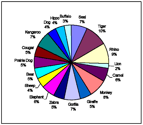
With all of the data collected, we found the percentages of the different animals. With that percent we made a pie chart and a bar chart. The attached pie chart shows the percents of the different animals. The bar chart shows the different animals in what each of their mean values are. Also, we were able to figure the probability of selecting each animal out of 10 selections.

We used page 40 of our textbook to come up with a confidence statement. We are 95% confident that the true percentage of all animals in a small box of Nabisco animal crackers is Seal-7%, Tiger-10%, Rhino-9%, Lion-2%, Camel-6%, Monkey-8%, Giraffe-5%, Gorilla-7%, Zebra-5%, Elephant-6%, Sheep-4%, Bear-5%, Prairie Dog-5%, Cougar-5%, Kangaroo-7%, Dog-4%, Hippo-4%, and Buffalo-3% + or – 3 percentage points. Our margin of error would have been smaller if we used a larger sample.

In conclusion we were able to determine the distribution of each animal. Due to the number of variables and small sample size it is difficult to determine whether or not our study is accurate in the real world sense. We accepted a null hypothesis because we found nothing interesting occurring.

Average Age of Death Comparison

What is the average age of death for both males and females buried at Mt. Vernon Cemetery? This was the question we decided to answer with our project. We chose this particular question to answer because we had an interest in finding out whether the recent statistic of females living longer than males was true here. We also wanted to see if the average age of death was between 50 and 70 years old for males and 60 and 80 years old for females. In our project the variables were the ages of death for females and the ages of death for males at Mt. Vernon Cemetery. The explanatory variable was the year of birth and year of death of each male and female and the response variable was the ages of death of each that determined the average. The details of this data collection process will be explained throughout this paper.

Our group had very busy schedules, so it was hard to do the data collection process together, so we were each assigned a section of the six already marked sections. We each mapped and assigned all the headstones with a number (first males, then females). After this, we each took the total number of the section and multiplied by .05. This gave each of us how many headstones to use in the random selection for the 5% sample. (Note: each section differed in the total number of headstones, therefore each section differed in how many headstones were to be used in the sample.) We used the table out of our statistics book to randomly pick the headstones to be recorded. After doing this, we each added up the ages of death, and then divided by the number of selected headstones to get the male/female average for each section.

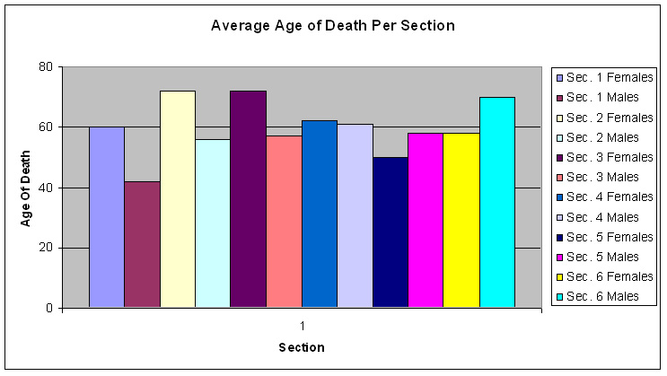
With all of our data collected we were able to look at the averages within each section and compare the average age of death for both males and females. The following graph shows the averages for sections 1–6:

We chose the bar graph because of its ability to clearly compare variables. As you can see, if one were to look at this graph, section wise, the females, on average, seem to have lived longer than males except within the last two sections. Also, one would think that we were right in assuming that the average age of death was between 50 and 70 for males and between 60 and 80 for females. Understand that this was kind of like a first draft, and we actually thought that we had answered our question with it. What we missed at the time, was the fact that we needed to compile the data into one big section to obtain the overall average in the cemetery with the sample we randomly selected. The following graph conveys the real results well:

Our original question of “what is the average age of death of both males and females?” was answered by using the box plot graph, which displays the median, quarter 1, quarter 3, high and low of data collected. This graph proved us wrong twice. At Mt. Vernon Cemetery, the average age of death for females is not between 60 and 80. It is actually between 48.34 and 68.18 years old. Also, on average, as displayed in this graph, males seem to live longer than females. Another thing this graph shows is just the average age of death at Mt. Vernon Cemetery for curiosity purposes.

This may not be 100% accurate, though, because we have to allow for human error in the recording process. Some headstones were unreadable and others either had no birth date, no death date, or both. But we had to include them as not to seem bias in the population. As for the sample, we ensured accuracy by agreeing to randomly select accuracy, in the data analysis, the probability of our Ho (the mean for males = the mean for females) was calculated. The result was a .6, which means that if someone else did this study, the same overall results would have been found 60% of the time compared to the Hi (male mean does not equal female mean). And to be a little more sure in our data, we had the probability calculated that each section had the same mean. We found that p = .676. This insures the integrity of our study.

With all this in mind, we are 95% confident that males, on average, live longer than females at Mt. Vernon Cemetery, Peru, Nebraska, and the average age of death is between 53.92 and 69.17 (50 and 70) for males, and between 48.34 and 68.18 (40 and 70) and not 60 and 80 for females.

2004 McGraw-Hill Higher Education
Any use is subject to the Terms of Use and Privacy Policy.
McGraw-Hill Higher Education is one of the many fine businesses of The McGraw-Hill Companies.