Questions 10-3 to 10-5 refer to the graph below.
 |
| 3 | |
 <a onClick="window.open('/olcweb/cgi/pluginpop.cgi?it=jpg::::/sites/dl/free/0073375942/236468/chap10_1.jpg','popWin', 'width=NaN,height=NaN,resizable,scrollbars');" href="#"><img valign="absmiddle" height="16" width="16" border="0" src="/olcweb/styles/shared/linkicons/image.gif"> (5.0K)</a> <a onClick="window.open('/olcweb/cgi/pluginpop.cgi?it=jpg::::/sites/dl/free/0073375942/236468/chap10_1.jpg','popWin', 'width=NaN,height=NaN,resizable,scrollbars');" href="#"><img valign="absmiddle" height="16" width="16" border="0" src="/olcweb/styles/shared/linkicons/image.gif"> (5.0K)</a>
In the graph above the ATC and the AVC converge as quantity increases because |
| | A) | total fixed costs fall as output increases. |
| | B) | Total variable costs rise as output increases but total fixed costs stay constant, thus AFC falls and AVC rises. |
| | C) | Marginal costs pull up on the AVC curve but do not effect the ATC. |
| | D) | Both b and c are correct. |
|
|
|
| 4 | |
AVC begins to rise before ATC does because |
| | A) | AVC is not being pulled down by the declining AFC. |
| | B) | Diminishing returns in production effects the ATC but not the AVC. |
| | C) | The marginal cost curve impacts the AVC but not the ATC. |
| | D) | Of all of the above. |
| | E) | None of the above. |
|
|
|
| 5 | |
Which of the following statements is not true of the cost curves graphed above? |
| | A) | The functions are derived from a production function that exhibits increasing and then decreasing returns to production. |
| | B) | Average fixed cost could be derived from the functions shown. |
| | C) | The ATC includes only explicit accounting costs of production. |
| | D) | If just the MC were given for each unit of output, then the total variable and average variable cost could be calculated. |
|
|
|
| 6 | |
When choosing which plant to use for the production of increased output one must know which of the following information? |
| | A) | The ATC function of each plant. |
| | B) | The AFC function of each plant. |
| | C) | The MC function of each plant. |
| | D) | More than one of the above. |
|
|
|
| 7 | |
Based on the production function and isocost curve graphed below where the firm is operating at point A, we can say that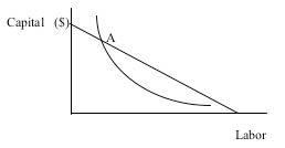 <a onClick="window.open('/olcweb/cgi/pluginpop.cgi?it=jpg::::/sites/dl/free/0073375942/236468/chap10_2.jpg','popWin', 'width=NaN,height=NaN,resizable,scrollbars');" href="#"><img valign="absmiddle" height="16" width="16" border="0" src="/olcweb/styles/shared/linkicons/image.gif"> (3.0K)</a> <a onClick="window.open('/olcweb/cgi/pluginpop.cgi?it=jpg::::/sites/dl/free/0073375942/236468/chap10_2.jpg','popWin', 'width=NaN,height=NaN,resizable,scrollbars');" href="#"><img valign="absmiddle" height="16" width="16" border="0" src="/olcweb/styles/shared/linkicons/image.gif"> (3.0K)</a>
|
| | A) | The firm could produce more without raising cost by hiring more labor and buying less capital. |
| | B) | The firm could produce more without raising cost by buying more capital and hiring less labor. |
| | C) | The firm could produce the same amount and lower costs by hiring more labor and buying less capital. |
| | D) | The firm could produce the same amount and lower costs by hiring less labor and buying more capital. |
| | E) | More than one of the above is correct. |
|
|
|
| 8 | |
In the graph shown in 10-7 above at point A |
| | A) | the MPL /MPK = PL/PK |
| | B) | The MPL /MPK > PL/PK |
| | C) | The MPL /MPK < PL/PK |
| | D) | The MPL /MPK = PK/PL |
|
|
|
| 9 | |
Long run cost curves for a firm |
| | A) | can be derived from the expansion path of a firm. |
| | B) | imply an optimal input combination for each output. |
| | C) | show the lowest possible cost for each possible output quantity. |
| | D) | are described in part by each one of the above answers. |
| | E) | are described in part by none of the above answers. |
|
|
|
| 10 | |
Which statement is not true about costs. |
| | A) | Economies of scale give rise to natural monopolies. |
| | B) | A small firm producing at the lowest point on its short-run ATC curve may have higher ATC costs than a larger firm producing at outputs less than the lowest point on its short-run ATC. |
| | C) | If the long run marginal cost is below the long run average total cost over the entire market output, then diseconomies of scale exist in the cost structure of that industry. |
| | D) | It is not possible for a firm to be operating efficiently if its short-run ATC curve is not tangent to the long-run ATC in the industry. |
|
|
|
| 11 | |
Given an output of 20, if average total cost is 80 and total fixed cost is 600, what is the average variable cost? |
| | A) | 50 |
| | B) | 80 |
| | C) | 1600 |
| | D) | 1000 |
| | E) | None of the above is correct. |
|
|
|
| 12 | |
Which statement is true? |
| | A) | There are no fixed costs in the long-run. |
| | B) | Average fixed costs are constant over the relevant range of output. |
| | C) | Marginal costs are unrelated to variable costs. |
| | D) | Total costs constantly rise over any relevant range of output. |
| | E) | Both a and d are correct. |
|
|
|
| 13 | |
Which of the following is not true about a set of average and marginal cost curves? |
| | A) | The marginal cost curve intersects the average variable cost curve at its lowest point. |
| | B) | The marginal cost curve intersects the average total cost curve at its minimum point. |
| | C) | The average variable cost curve reaches a minimum at a lower output than does the average total cost curve. |
| | D) | The marginal cost curve never declines in a typical graph of typical cost curves. |
|
|
|
| 14 | |
If the marginal cost curve of one factory is MC = 10Q and a second factory producing the same product has a MC = 15Q, then if you want to produce 25 units of output you should produce ___ in factory 1 and ____ in factory 2. |
| | A) | 25, 0 |
| | B) | 15, 10 |
| | C) | 0, 25 |
| | D) | It is impossible to tell without average cost information how much should be produced where. |
|
|
|
| 15 | |
Your textbook uses the following equation to describe an isocost line. (C = rK + wL) In this equation the |
| | A) | r is the unit cost of capital. |
| | B) | w is the number of labor units employed. |
| | C) | C is the per unit cost of output. |
| | D) | L is the wage rate of labor. |
| | E) | Answers above are all correct. |
|
|
|
| 16 | |
In the graph below which of the following is true?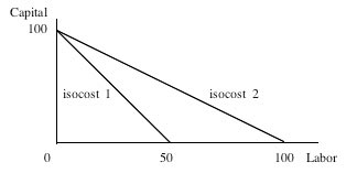 <a onClick="window.open('/olcweb/cgi/pluginpop.cgi?it=jpg::::/sites/dl/free/0073375942/236468/chap10_3.jpg','popWin', 'width=NaN,height=NaN,resizable,scrollbars');" href="#"><img valign="absmiddle" height="16" width="16" border="0" src="/olcweb/styles/shared/linkicons/image.gif"> (5.0K)</a> <a onClick="window.open('/olcweb/cgi/pluginpop.cgi?it=jpg::::/sites/dl/free/0073375942/236468/chap10_3.jpg','popWin', 'width=NaN,height=NaN,resizable,scrollbars');" href="#"><img valign="absmiddle" height="16" width="16" border="0" src="/olcweb/styles/shared/linkicons/image.gif"> (5.0K)</a>
|
| | A) | Along isocost line 2 production costs are higher than along isocost line 1. |
| | B) | Labor is more expensive per unit along isocost line 1 than along isocost line 2. |
| | C) | Capital is more expensive per unit than labor along isocost line 2. |
| | D) | If you were a producer that had a choice of either isocost lines above, you would most likely choose isocost line 1 because it is more efficient. |
|
|
Refer to the graph below consisting of 3 isoquants and 2 isocost curves for questions 17 and 18.