 <a onClick="window.open('/olcweb/cgi/pluginpop.cgi?it=jpg::::/sites/dl/free/0073451342/295036/ch06.jpg','popWin', 'width=NaN,height=NaN,resizable,scrollbars');" href="#"><img valign="absmiddle" height="16" width="16" border="0" src="/olcweb/styles/shared/linkicons/image.gif"> (24.0K)</a> <a onClick="window.open('/olcweb/cgi/pluginpop.cgi?it=jpg::::/sites/dl/free/0073451342/295036/ch06.jpg','popWin', 'width=NaN,height=NaN,resizable,scrollbars');" href="#"><img valign="absmiddle" height="16" width="16" border="0" src="/olcweb/styles/shared/linkicons/image.gif"> (24.0K)</a> |
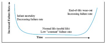
Electronics companies constantly test their products for reliability. A small change in the reliability of a component can make or break the sales of a product. The lifetime of an electronics component is often viewed as having three stages, as illustrated by the so-called bathtubcurve shown in the figure.
This curve indicates the average failure rate of the product as a function of age. In the first stage (called the infant mortality phase), the failure rate drops rapidly as faulty components quickly fail. If the component survives this initial phase, it enters a lengthy second phase (the usefullife phase) of constant failure rate. The third phase shows an increase in failure rate as the components reach the physical limit of their lifespan.
The constant failure rate of the useful life phase has several interesting consequences. First, the failures are "memoryless" in the sense that the probability that the component lasts another hour is independent of the age of the component. A component that is 40 hours old may be as likely to last another hour as a component that is only 10 hours old. This unusual property holds for electronics components such as lightbulbs, during the useful life phase.
 <a onClick="window.open('/olcweb/cgi/pluginpop.cgi?it=jpg::::/sites/dl/free/0073451342/295036/ch06_chart.jpg','popWin', 'width=NaN,height=NaN,resizable,scrollbars');" href="#"><img valign="absmiddle" height="16" width="16" border="0" src="/olcweb/styles/shared/linkicons/image.gif"> (9.0K)</a> <a onClick="window.open('/olcweb/cgi/pluginpop.cgi?it=jpg::::/sites/dl/free/0073451342/295036/ch06_chart.jpg','popWin', 'width=NaN,height=NaN,resizable,scrollbars');" href="#"><img valign="absmiddle" height="16" width="16" border="0" src="/olcweb/styles/shared/linkicons/image.gif"> (9.0K)</a> <a onClick="window.open('/olcweb/cgi/pluginpop.cgi?it=jpg::::/sites/dl/free/0073451342/295036/ch06_integral.jpg','popWin', 'width=NaN,height=NaN,resizable,scrollbars');" href="#"><img valign="absmiddle" height="16" width="16" border="0" src="/olcweb/styles/shared/linkicons/image.gif"> (1.0K)</a> <a onClick="window.open('/olcweb/cgi/pluginpop.cgi?it=jpg::::/sites/dl/free/0073451342/295036/ch06_integral.jpg','popWin', 'width=NaN,height=NaN,resizable,scrollbars');" href="#"><img valign="absmiddle" height="16" width="16" border="0" src="/olcweb/styles/shared/linkicons/image.gif"> (1.0K)</a>
for some constant c > 0. Before we evaluate this, we will need to extend our notion of integral to include improper integrals such as this, where one or both of the limits of integration are infinite. We do this in section 6.6. Another difficulty with this integral is that we do not presently know an antiderivative for f (x) = xe-cx . In section 6.2, we introduce a powerful technique called integration by parts that can be used to find antiderivatives of many such functions. The new techniques of integration introduced in this chapter provide us with a broad range of tools used to solve countless problems of interest to engineers, mathematicians and scientists.
|