Case Problems

Download as a Word document: Case Problems Ch01 (78.0K)

To practice working with text, values, and formulas, ensure that Excel is loaded and then display a blank workbook. You will begin by entering a Title ("Hancock Industries Monthly Budget" and subtitle ("Prepared By:" and include your name) for the worksheet. In the same row, in column F, enter the current date. Now enter the following categories and a reasonable amount for each, starting in Cell A5:

• Revenue (Press [Enter] twice before entering the next label)
• Expenses (Do not enter a value for this label)
• Materials
• Labor
• Overhead
• Total Expenses (do not enter a value for this row, you will enter a formula later)
• Net Income (do not enter a value for this row, you will enter a formula later)

In the cell to the right of the label "Total Expenses" enter a formula that sums (Adds up) the values you entered for Materials, Labor, and Overhead. Next enter a formula to subtract the Total Expenses value FROM the Revenue value.

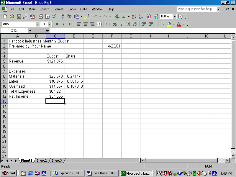
For the Expenses: Materials, Labor, and Overhead, enter a formula which calculates the percent of each item to the Total Expense. For example, you would divide the value for Materials by the value of Total Expenses. Figure 1-4 shows an example of the completed worksheet. Experiment by changing the values for Revenue, Materials, Labor and Overhead. What happens to the results of the formulas when you change these values?

<a onClick="window.open('/olcweb/cgi/pluginpop.cgi?it=gif:: ::/sites/dl/free/0072470941/26807/Ch01_Image1cp.gif','popWin', 'width=NaN,height=NaN,resizable,scrollbars');" href="#"><img valign="absmiddle" height="16" width="16" border="0" src="/olcweb/styles/shared/linkicons/image.gif"> (50.0K)</a>

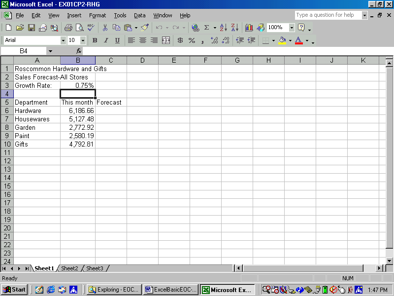
When completed, save the file as "HI-Budget" to your personal storage location.

Roscommon Hardware and Gifts

1. Open the file "EX01CP-RHG" to display the workbook shown in Figure 1-5.
   
   <a onClick="window.open('/olcweb/cgi/pluginpop.cgi?it=gif:: ::/sites/dl/free/0072470941/26807/Ch01_Image2cp.gif','popWin', 'width=NaN,height=NaN,resizable,scrollbars');" href="#"><img valign="absmiddle" height="16" width="16" border="0" src="/olcweb/styles/shared/linkicons/image.gif"> (50.0K)</a>
   
   
2. Save the file as "Forecast" to your personal storage location.
3. In column C "Forecast" increase each departments’ sales by the growth factor in cell C3. Use the cell reference in the formula, not the value. Check that you have the correct formula, is the forecast value more than the value for "This Month?" If not, you have an error in the formula and should try to fix it.
4. Calculate the total for each column and add an appropriate label in column A.
5. Change the growth rate from .75% to .57%. What effects did this have on your calculated values?
6. Change the label "This Month" in cell B5 to "April ‘01" and the label "Forecast" in cell C5 to "May ‘01".
7. Save the changes and close Excel.

Data File: EX01CP_RHG (13.0K)