 |  Statistics for the Behavioral Sciences, 4/e Michael Thorne,
Mississippi State University -- Mississippi State
Martin Giesen,
Mississippi State University -- Mississippi State
Chi Square
SPSS ExercisesUSING SPSS-EXAMPLES AND EXERCISES
SPSS has procedures for performing the chi-square goodness-of-fit test and the chi-square test of
independence between two categorical variables. However, SPSS is designed for use with raw data. The
data presented for the exercises in this chapter are in summary form. As a consequence, in order to use
SPSS, we must "unsummarize" the data- reconstruct the data as if they came from individual participants.
Unfortunately, the process of creating the data file will be somewhat laborious, and you may decide that it's
easier to work the problems using a hand calculator than using SPSS. In spite of the difficulties, you will
gain experience that will allow you to perform the chi-square-based tests using SPSS on data in the form
you would obtain in an actual research setting.Example - Chi-Square Goodness-of-Fit Test: To illustrate this technique, we will work Problem 7 using
SPSS. The steps are as follows:- Start SPSS and name the first variable grade. We must simulate the grade data for 170 students. Use the code numbers 4 for A, 3 for B, 2 for C, 1 for D, and 0 for F. Because there were 25 As, 35 Bs, 60 Cs, 30 Ds, and 20 Fs, you should enter 4 twenty-five times, 3 thirty-five times, and so on. (Hint: Use the editing features of the Windows environment to help. For example, enter 4 five times, copy the block, and paste it below each successive block until you reach 25. Do the same for the other numbers in blocks of 5 or 10 depending on the totals needed.)
- Select Analyze > Nonparametric Tests > Chi-Square.
- Move grade into the Test Variable List box.
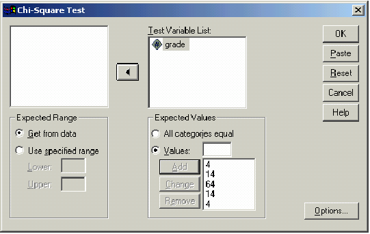
- We now need to tell SPSS what our expected frequencies ratio is, if it is something other than an equal proportion for each group. In the Expected Values box, select Values and enter 4 (for 4%) in the entry box, then click Add. Repeat this process in order for all five expected value percentages: 4, 14, 64, 14, and 4. The resulting dialog box should appear as follows. Click OK and the results should appear in the output Viewer window.
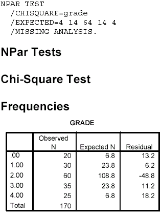
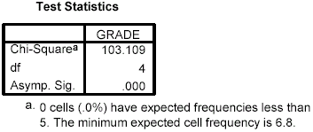
 <a onClick="window.open('/olcweb/cgi/pluginpop.cgi?it=gif:: ::/sites/dl/free/0072832517/55323/c14_spss1.gif','popWin', 'width=NaN,height=NaN,resizable,scrollbars');" href="#"><img valign="absmiddle" height="16" width="16" border="0" src="/olcweb/styles/shared/linkicons/image.gif"> (17.0K)</a> Notes on Reading the Output <a onClick="window.open('/olcweb/cgi/pluginpop.cgi?it=gif:: ::/sites/dl/free/0072832517/55323/c14_spss1.gif','popWin', 'width=NaN,height=NaN,resizable,scrollbars');" href="#"><img valign="absmiddle" height="16" width="16" border="0" src="/olcweb/styles/shared/linkicons/image.gif"> (17.0K)</a> Notes on Reading the Output- You should find the output easy to read and understand. The observed frequency, expected frequency, and difference (labeled Residual) are given in the first box and the test statistics in the second box. The results indicate that the actual grade assignment does differ significantly from a normal distribution: c2 (4, N = 170) = 103.11, p < .001.
 <a onClick="window.open('/olcweb/cgi/pluginpop.cgi?it=gif:: ::/sites/dl/free/0072832517/55323/c14_spss2.gif','popWin', 'width=NaN,height=NaN,resizable,scrollbars');" href="#"><img valign="absmiddle" height="16" width="16" border="0" src="/olcweb/styles/shared/linkicons/image.gif"> (10.0K)</a> <a onClick="window.open('/olcweb/cgi/pluginpop.cgi?it=gif:: ::/sites/dl/free/0072832517/55323/c14_spss2.gif','popWin', 'width=NaN,height=NaN,resizable,scrollbars');" href="#"><img valign="absmiddle" height="16" width="16" border="0" src="/olcweb/styles/shared/linkicons/image.gif"> (10.0K)</a>  <a onClick="window.open('/olcweb/cgi/pluginpop.cgi?it=gif:: ::/sites/dl/free/0072832517/55323/c14_spss3.gif','popWin', 'width=NaN,height=NaN,resizable,scrollbars');" href="#"><img valign="absmiddle" height="16" width="16" border="0" src="/olcweb/styles/shared/linkicons/image.gif"> (6.0K)</a> Example - Chi-Square Test of Independence:
We will use SPSS to work Problem 6. Let's shorten the
data entry required for this problem by taking half of the frequency for each condition to result in an N = 80
rather than 160. The steps are as follows: <a onClick="window.open('/olcweb/cgi/pluginpop.cgi?it=gif:: ::/sites/dl/free/0072832517/55323/c14_spss3.gif','popWin', 'width=NaN,height=NaN,resizable,scrollbars');" href="#"><img valign="absmiddle" height="16" width="16" border="0" src="/olcweb/styles/shared/linkicons/image.gif"> (6.0K)</a> Example - Chi-Square Test of Independence:
We will use SPSS to work Problem 6. Let's shorten the
data entry required for this problem by taking half of the frequency for each condition to result in an N = 80
rather than 160. The steps are as follows:- Start SPSS and name variables ie and pref. Use a code value of 1 for introverts and 2 for extraverts; use 1 for Brand A, 2 for Brand B, and 3 for Brand C. You will need 21 entries for introverts preferring Brand A (ie = 1 and pref = 1), and so on. The data entry window should show a pattern like this: 1, 1 for 21 entries; 2, 1 for 18 entries; 1, 2 for 9 entries; 2, 2 for 8 entries; 1, 3 for 10 entries; and 2, 3 for 14 entries.
- Select Analyze>Summarize>Crosstabs.
- In the dialog box, move ie into the Rows box and pref into the Columns box. Select the Statistics box, then Chi-Square>Continue.
- Also select the Cells box-in the Counts box, Observed should be checked by default; also check Expected. In the Percentages box, click Total, then Continue and OK. The results should appear in the output Viewer window.
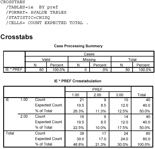
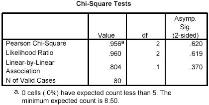
Notes on Reading the Output- The IE*PREF Crosstabulation box shows the frequency (count) for each cell. Note that in each cell, the first number is the frequency, the second is the expected frequency, and the third number is the percentage for that cell based on the cell frequency divided by the total sample size. If you look at the percentages across the brand preference groups, you will see that there is not much difference in the pattern between introverts and extraverts. Both prefer Brand A, then Brand C, and Brand B least.
- Shown in the Chi-Square Tests box, the Pearson Chi-Square value is 0.956, with p = .62. Thus, the results indicate that introversion or extraversion does not make a difference in brand preference: c2 (2, N = 80) = 0.956, p = .62.
 <a onClick="window.open('/olcweb/cgi/pluginpop.cgi?it=gif:: ::/sites/dl/free/0072832517/55323/c14_spss4.gif','popWin', 'width=NaN,height=NaN,resizable,scrollbars');" href="#"><img valign="absmiddle" height="16" width="16" border="0" src="/olcweb/styles/shared/linkicons/image.gif"> (20.0K)</a> <a onClick="window.open('/olcweb/cgi/pluginpop.cgi?it=gif:: ::/sites/dl/free/0072832517/55323/c14_spss4.gif','popWin', 'width=NaN,height=NaN,resizable,scrollbars');" href="#"><img valign="absmiddle" height="16" width="16" border="0" src="/olcweb/styles/shared/linkicons/image.gif"> (20.0K)</a>  <a onClick="window.open('/olcweb/cgi/pluginpop.cgi?it=gif:: ::/sites/dl/free/0072832517/55323/c14_spss5.gif','popWin', 'width=NaN,height=NaN,resizable,scrollbars');" href="#"><img valign="absmiddle" height="16" width="16" border="0" src="/olcweb/styles/shared/linkicons/image.gif"> (10.0K)</a> Exercises Using SPSS <a onClick="window.open('/olcweb/cgi/pluginpop.cgi?it=gif:: ::/sites/dl/free/0072832517/55323/c14_spss5.gif','popWin', 'width=NaN,height=NaN,resizable,scrollbars');" href="#"><img valign="absmiddle" height="16" width="16" border="0" src="/olcweb/styles/shared/linkicons/image.gif"> (10.0K)</a> Exercises Using SPSS- Use SPSS to work Problem 9. There should be 28 data entries, with a value of 1 for 23 and 0 for the remaining 5. Chance prediction would be that being above or below the departmental average would be equally likely; thus, the expected frequencies would be equal. This is the default in the Chi-Square Test dialog box. For Expected Values, All Categories Equal already should be checked and is the appropriate setting for this exercise. Write a conclusion.
- Use SPSS to perform a chi-square test of independence using the data from Problem 8. Name the variables esteem and risk. Use a code of 1 for low self-esteem and 2 for high self-esteem; use a code of 1 for low risk takers and 2 for high risk takers. You will need to enter data for 60 participants. Write a conclusion.
 Click here to view the answers. (114.0K) Click here to view the answers. (114.0K)
|
|


 2003 McGraw-Hill Higher Education