Hands-On Exercises

Download as a Word document: Hands-On Exercises Ch05 (198.0K)

Sunny Side Marina: Aging Accounts Receivable

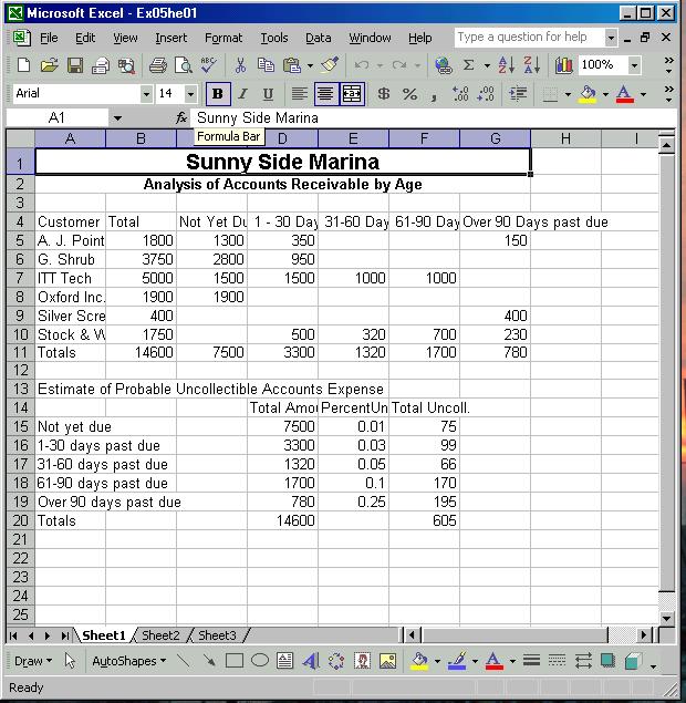
In this exercise you will practice working with draw objects, formatting and styles.

Open the data file named EX05HE01. Your screen should look like Figure 5-1.

Save the workbook as "Aging" to your personal storage location.

Figure 5-1

The first change is to select cells C4 through G4.
SELECT: Cell C4:G4

Now you need to have the text in the cells wrap within the cells to display the whole string.
CHOOSE: Format, Cells, if not already selected click the Alignment tab
CLICK: the Check box next to Wrap Text

On your own, wrap the text in cells D14 through F14.

The next step is to apply an AutoFormat to Cells C4 through G11. You will let Excel choose the range.
SELECT: Cell C4
CHOOSE: Format, AutoFormat…
SCROLL: Through the options until you find Accounting 3
CLICK: Accounting 3
CLICK: [Options…] button. Review the options, but don’t make any changes at this time
CLICK: [OK] button

On your own, merge and center the label in cell A13 across cells A13 to G13. Format it to appear similar to the label in row 2. (Hint: you can use the format painter.)

Next you will format the Estimate of Probable Uncollectible Accounts Expense.
SELECT: Cells A15 to A19
CHOOSE: Format, Cells. Click the alignment tab
CLICK: the Indent spin control three times (The text box should read 3)
CLICK: [OK] button
SELECT: Cell A20
CHOOSE: Format, Cells

CLICK: the alignment tab
CLICK: the Indent spin control five times. (The text box should read 5)
CLICK: [OK] button

Lastly, you will apply number styles and boarders to the table manually (do not use the AutoFormat feature).
SELECT: Cells D15, F15, D20, and F20 (after selecting cell D15, hold down the [Ctrl] key to select each additional cell)
CLICK: [$] style button on the Formatting tool bar
SELECT: Cell range D16:D19, and F16:F19 using same technique as above
CLICK: [,] style button on the Formatting tool bar
SELECT: Cell range E15:E19
CLICK: [%] style button
SELECT: Cells D20 and F20
CLICK: Boarders drop down arrow, and choose Top and Double Bottom Border

PRESS: [Ctrl] + [Home],
Save your work, and close Excel.

Data File: EX05HE01 (14.0K)

Turtle River Casinos-Performance Analysis

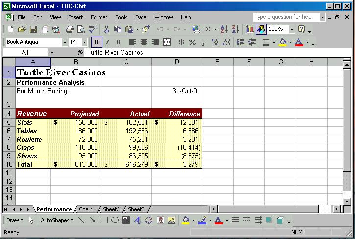
In this exercise you will practice creating and customizing charts.

Open the data file named EX05HE02. Your screen should appear similar to Figure 5-2.

Figure 5-2

Save the workbook as "Performance" to your personal storage location.

Review the workbook and familiarize yourself with the data. After reviewing the performance sheet…
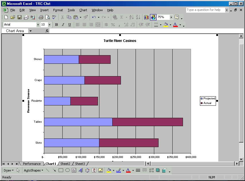
CLICK: Chart 1 tab (Figure 5-3)

Figure 5-3

First, you are asked to change the chart type.
CLICK: Chart, Chart Type…
CHOOSE: "Clustered column with a 3-D visual effect" (second row, first column)
CLICK: [OK] button

Delete both axis titles
CLICK: Chart, Chart Options…
DELETE: entries in the Category (X) axis text box, and the Value (Y) axis text box
CLICK: OK

Switch back to the Performance Analysis.
CLICK: Performance tab

You are asked to prepare a chart for investor, which shows the breakdown of the actual revenue, by type. On your own, select nonadjacent cell ranges A5:A9 and D5:D9, Then:
CLICK: Chart wizard button
CHOOSE: Pie chart type
CHOOSE: Pie with a 3-D visual effect
CLICK: Next 2 times

In step 3 of 4, Chart options dialog box,
TYPE: Actual Revenue for October in the Chart title text box.
CLICK: Legend Tab
CLICK: Show legend check box to remove the check mark
CLICK: Data Labels tab
CLICK: Category name check box (to add a check mark)
CLICK: Next

In step 4 of 4, Chart location:
CLICK: As new sheet radio button
TYPE: Actual Performance in the sheet name text box
CLICK Finish

Since this is to be used for a presentation, someone suggests that you use Word Art to create the title for the chart. But first you need to delete the existing title:
SELECT: Actual Revenue for October
PRESS: Delete
(If the drawing tool bar isn’t on your screen, do the following)
CLICK: View, Toolbars, Drawing
CLICK: Insert WordArt on the drawing toolbar
SELECT: a word art style
CLICK: OK
TYPE: Actual Performance for October
CLICK: [OK] button

On your own, reposition the new title so it is not covering the chart.

If you have a printer attached, print the chart and the worksheet together (Hold down the control key and select both tabs)

Save and close the file. Exit Excel.

Data File: EX05HE02 (16.0K)

2002 McGraw-Hill Higher Education
Any use is subject to the Terms of Use and Privacy Policy.
McGraw-Hill Higher Education is one of the many fine businesses of The McGraw-Hill Companies.